Network-based assignment of RNA-binding protein function

TL;DR

This project aims to identify the functionalities of RNA-binding proteins (RBPs) through proteomics data and network analysis. Mass-spectrometry data was used to collect interaction partners for 40 RBPs with known functionalities in mRNA life cycle. Then, a network was constructed to connect all the proteins, and a guilt-by-association principle was applied to assign novel functionalities. As a result, a Shiny app database https://butterlab.imb-mainz.de/RINE/ was created for interactive data exploration. If you find the app interesting and want to learn more about the data analysis behind it, please continue reading.

Introduction

This project is the foundation of my PhD thesis, which focuses on mass-spectrometry (MS) data, specifically on RNA-binding proteins (RBPs) and their associated functionalities. In recent years, the number of proteins classified as RBPs has skyrocketed, with 1,273 proteins classified as RBPs in yeast alone. If you’re curious about this phenomenon, you can check out this informative review by Hentze et al. Despite the increasing number of proteins classified as RBPs, their functional roles remain largely unexplored.

The main reason behind this lack of functional details is that newly described RBPs mostly come from high-throughput techniques such as RNA interactome capture (RIC). These techniques generate large datasets and excel at identifying and classifying individuals, but they lack deep biological characterization. The goal of this project was to add a first layer of functional characterization while maintaining a high-throughput approach. Therefore, we selected 40 well-characterized yeast RBPs and identified their interaction partners with immunoprecipitation coupled to MS-based quantitative proteomics. With this data, we were able to build function-based networks to gather hints on which individuals might be involved in particular RNA-related pathways.

The Data

Candidate RBPs

To begin with, I aimed to gather the interaction partners of 40 chosen RBPs, which would serve as the foundation of our function-based networks. Before delving into the interactors data, let’s take a step back and examine the candidates data. Why specifically these 40 RBPs? How do they facilitate the formation of function-based networks? Moreover, what precisely do I mean by “function-based networks”?

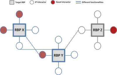
Let’s start by refreshing some basic network terminology. In this post, I will refer to the selected RBPs as “network hubs”, their interaction partners as “nodes”, and the connections between them as “edges”. By using this terminology, each square representing a target RBP can be considered a hub, each circle representing an IP interactor can be considered a node, and the lines representing connections between them can be considered edges. Using these three elements, I created the RBP interactome network. When we later filter this larger network for a particular functionality, we obtain a “function-based network”. For example, if we only keep the blue hubs, we can create a blue function-based network.

With our network lingua franca established, let’s now focus on our 40 RBP candidates. These RBPs were selected based on their potential to become the hubs on the function-based networks. To ensure this, it was crucial to choose well-studied candidates that play central roles in their pathways. To identify such candidates, I consulted the KEGG and Reactome databases, which helped me identify RBPs involved in RNA biology pathways such as degradation or splicing. Additionally, our candidates needed to be included in the TAP-tagged commercial library so that I could capture them with an antibody.

Interactors data

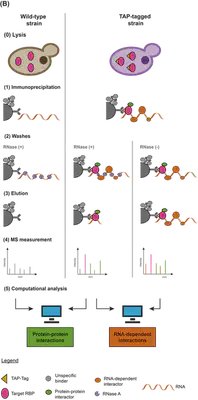
I performed immunoprecipitation on each of the selected RBPs and captured all their interacting partners in the presence or absence of RNA. This allowed me to obtain two distinct groups of interactors:

• Protein-Protein interactors (PPI): As a result of RNA digestion by RNase A, all the nodes in this group interact with our hubs in an RNA-independent manner.
• RNA-dependent interactors (RDI): This group consists of all the nodes that interact with our hubs in an RNA-dependent manner.

Using a label-free quantification (LFQ) MS protocol, I quantified the interactors in both groups. These interactors, along with the hub candidates, served as the building blocks for constructing the function-based networks.

Data analysis

I have not included any code on this post but, If you get curious and want to check it, you can find it available at the following github repository github repository. I will reference which subfolders belong to each analysis on their corresponding subsection.

RBP interactors quantification

The code for this analysis can be found in the following github repository subfolder. During this section, I am gonna assume you know some basic MS concepts; otherwise you can check this nice review from Sinha et al. to freshen them up.

After the immunoprecipitation experiments, I obtained, in quadruplicate, protein elution products for three conditions:

• Wild type (WT)
• TAP-tagged IP RNase treated (RNase)
• TAP-tagged IP untreated (IP) These are ready for MS measurement; as mentioned before, I choose a LFQ protocol. Long story short, this means we can directly use our digested peptides without adding any chemical or metabolic labelling. This way, for each of our selected 40 candidates I would quantify their RNase and IP interactors so I could compare them to each other and against a WT. The first step in the quantification is to match the MS peptide spectra with protein groups; for this purpose, I use the andromeda search engine as incorporated in MaxQuant. This allows for protein quantification, based on the peptide intensity. I will not go into further details on how LFQ works, you can chek this review from Cox et al. if you want to learn more.

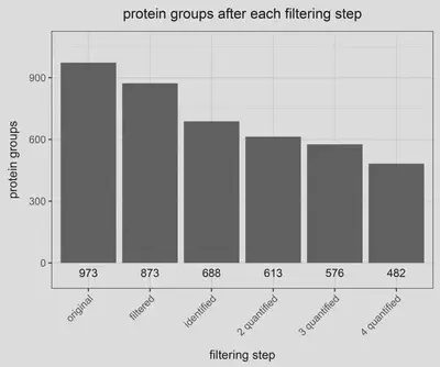
With our proteins identified we proceed with a series of quality control filtering steps; mainly we filter out the following protein groups:

• Known contaminants, present on any MS experiment (i. e., keratin), as provided by the Cox lab
• Reverse peptides
• Filter peptides by razor and unique peptide number. This way, I only keep protein with a minimum of razor+unique peptide count higher than 2 and a minimum of unique peptide count higher than 1.
• Filter out by quantification event. This way, I decide to keep only proteins with a minimum of 2 quantification events along the replicates. Thus, any protein without an intensity value associated (not NA) in, at least, two out of four replicates will be filtered out.

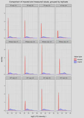
Next step is dealing with the missing values. A known issue of MS experiments is the abundance of NA values along the detected protein groups due to technical limitations. For instance, a protein group could be identified with an average intensity of 25 in three replicates and have an NA value on the fourth. Our approach for these NA values is to assume that the protein was not detected due to technical limitations not because it was not present in the protein mixture. This way, we decide to impute an intensity value for all NA values still present after the filtering steps. We do so by shifting a beta distribution obtained from the LFQ intensity values to the limit of quantitation. This way, the resulting imputed values will always be random values constricted to the lowest end of our LFQ intensities. This is just one approach among many; if you are interested in further reading regarding MS data imputation, I would suggest this article from Wei et al.. With our NA values imputed, we are ready to proceed with a series of quality control and exploratory analysis checks. These are pretty standard on any omics analysis (i. e., clustering by pearson correlation coefficient and dimensionality reduction by PCA) so I will not cover them in this post.

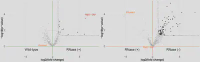
This leads to our final step, where we assess quantified interactors differences among our three conditions. We do so with a standard t-test. The results are visualised as a volcano plot, which offers an intuitive way to identify enriched interactors and benchmark the experiment quality by observing the RBP-TAP and RNase behaviour. As described before, we are interested in obtaining to groups of interactors, as shown for PAB1 in the example volcano plots:

• PPI, resulting from the comparison of a treated TAP-tagged RBP (RNase) to a wildt type (WT). In this comparison, the RBP-TAP targeted during the immunoprecipitation gets clearly enriched as it is not pulled down on the WT condition. On the other hand, the RNase enzyme falls on the background due to its presence in both conditions. All RBP-TAP RNA independent interactors get enriched in this comparison.
• RDI, resulting from the comparison of an untreated TAP-tagged RBP (IP) to a treated TAP-tagged RBP (RNase). In this comparison, the RBP-TAP targeted during the immunoprecipitation falls on the background as it is equally pulled down in both conditions. On the other hand, the RNase enzyme gets negatively enriched as it is only present in the treated condition (RNase). All RBP-TAP RNA dependent interactors get enriched in this comparison.

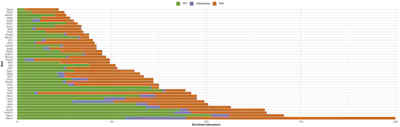
This way, we repeated this setup for all our 40 RBPs and we obtained two clearly different groups (minimal overlap, in purple on the barplot image) corresponding to the PPI and RDI.

Functional Analysis

The code for this analysis can be found in the following github repository subfolder.

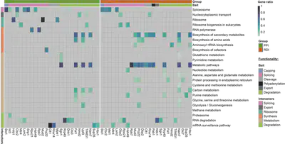
After the (long) quantification section, I described how our network hubs (target tagged RBPs) and nodes (PPI and RDI groups) were obtained. At this point I would be ready to build the interactome network, as the edges just connect the nodes to the hubs when they were quantified on their respective experiments. I indeed have all the elements to build a basic interactome network, but I am interested in building a function-based network. Thus I need to classify the hubs by function in order to do so. I already selected them following functional criteria and one could argue this would be already enough. But I want to take it a step further and see if not just the hubs have associated functions but also their associated nodes. Thus, I choose to perform a functional enrichment analysis for each hub associated nodes. Again, this is a standard analysis included on many omics workflows so I will not cover it deeply. Long story short, I performed an over-representation analysis as implemented in the ClusterProfiler R package which, in brief, calculates p-values by hypergeometric distribution from a experimentally derived list of enriched IDs (PPI or RDI groups) and its background (Quantified proteins). This way we obtained the PPI and RDI associated KEGG pathways for each hub, if any.

Network Analysis

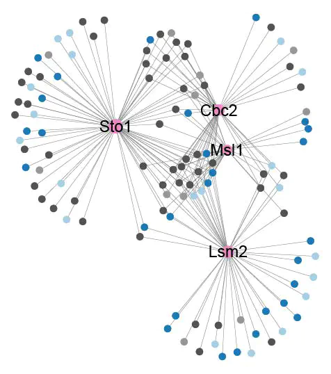
Now comes the fun part; I do have all the elements to construct a network (hubs, nodes and edges) and a data-driven functional classification criteria. Thus I can proceed to build the networks, with the R igraph nicely algorithm implementation. For the PPI and RDI data, I decided to create two different kind of networks:

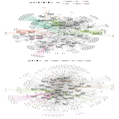
• A global network, containing all 40 hubs. In such networks, hubs and their edges would be colour highlighted when they had a unique associated function.

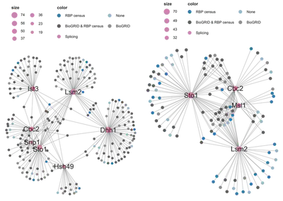
• A function-based subnetwork, containing all hubs associated with a particular subnetwork. For these networks I also colour highlighted the nodes, so they would show whether they have been reported before or not on the BioGRID database and whether they have been classified as RBPs or not.

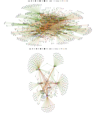
Additionally I also combined the PPI and RDI groups into a global network and function-based subnetwork. For these networks, instead of highlighting the hubs or the nodes I choose to highlight the edges to show their group association (PPI, RDI or overlap).

Conclusion

The purpose of all the data analysis and network building in this project is to create a valuable resource. We identified which nodes are novel, meaning they have not been reported in the BioGRID database, and whether they are classified as RBPs or not. Additionally, we identified potential functional associations with our function-based networks. Following the guilt-by-association principle, if a node is associated with other nodes and hubs that participate in splicing pathways, for example, it is likely involved in splicing. This can serve as a starting point for in-depth functional characterization. To facilitate this, I developed a user-friendly shiny app, available at https://butterlab.imb-mainz.de/RINE/, where all the networks can be explored. I hope this app makes the data accessible and enables RNA research labs to deepen their understanding of the RBP research field.