Interactive CV network
 My CV as a network
Table of Contents
TL;DR
The main idea behind this project is to make your CV shine, by visualizing its data and plotting it in an interactive fashion you. Thus what I want to do is to connect the usual entries on a CV (education, positions, publications…) by year, so I can visualize, in an intuitive way, how a career path has developed.
Thus our goal is to create an interactive network of the CV. If you would like to know how to generate something similar, continue to read.
Introduction
The inspiration for this network-plot is the fantastic package and tutorial datadrivencv, by Nick Strayer, which has the goal of automatizing the CV update. To do so, you would keep each entry on the CV on a .csv file that you would later render into a a .pdf or .html file. In such file, rows correspond to each entry on your CV, for instance your education degrees or job experiences, and columns describe the positions, for instance start year or location.
The data
The network-plot starting point is, this way, a CV entries data file. You can check out an example of a CV entries file at Nick’s Strayer tutorial spreadsheet. You can also download the necessary data to replicate this tutorial here.
For the network plot I just need each entry on the CV and its corresponding year, so I start by filtering our data with dplyr:
#Load entries data file:

my_df <- read.csv("network_entries.csv")

#Filter relevant columns:

my_relevant_df <- my_df %>% dplyr::select(title, start, end)
I want to make sure that all entries in start and end are numeric, as they should be years:
my_relevant_df$start <- as.numeric(my_relevant_df$start)

my_relevant_df$end <- as.numeric(my_relevant_df$end)
All non numeric entries (like empty values or years set to “current”) will be transformed into NA values. I will use this in our favour to further filter the data.
First I want to kick out all the rows containing NA both in start and end, as those are time independent entries (like skills) not relevant to network-plot:
#Flag NA values with the logic statement TRUE and combine columns start and year:

my_relevant_df$filter <- interaction(is.na(my_relevant_df$start),is.na(my_relevant_df$end))

#Filter out all entries that are "TRUE.TRUE" (NA values in both columns) and remove the filter columns:

my_relevant_df <- my_relevant_df[!my_relevant_df$filter == "TRUE.TRUE",]
my_relevant_df <- my_relevant_df %>% dplyr::select(title, start, end)
Our last step on data cleaning is assign year values to the remaining NA:
- NA values at the start column are assigned to be the same value that end year (i. e., a publication)
- NA values at the end column are assigned to current year (i. e., current job)
my_relevant_df <- my_relevant_df %>% dplyr::mutate(start = ifelse(is.na(start), end, start))

current_year <- lubridate::year(lubridate::ymd(Sys.Date()))
my_relevant_df <- my_relevant_df %>% dplyr::mutate(end = ifelse(is.na(end), current_year, end))
Now that the data is cleaned up, I will generate the two data frames I need for the network plot:
- Nodes data, containing each entry on the CV
- Edges data, containing the (year) connections among the CV entries
I start by generating the edges. First step is to assign a numeric id to each entry and selecting the year columns:
edges <- my_relevant_df
edges <- edges %>% dplyr::mutate(id = dplyr::row_number())
edges <- edges %>% dplyr::select(id, start, end)
Then I generate the edges with a function borrowed from the datadrivencv package:
#Combine the start and end years into a integer range
edges <- edges %>% purrr::pmap_dfr(function(id,
                         start, end) {
  dplyr::tibble(year = start:end, id = id)
})

#Nest all entries per year range
edges <-  edges %>% dplyr::group_by(year) %>% tidyr::nest() %>% dplyr::rename(ids_for_year = data)


#Generate the edges
combination_indices <- function(n) {
  rep_counts <- (n:1) - 1
  dplyr::tibble(a = rep(1:n, times = rep_counts), b = purrr::flatten_int(purrr::map(rep_counts,
                                                                                    ~{
                                                                                      tail(1:n, .x)
                                                                                    })))
}

edges <- edges %>% purrr::pmap_dfr(function(year, ids_for_year) {
  combination_indices(nrow(ids_for_year)) %>% dplyr::transmute(year = year,
                                                               from = ids_for_year$id[a], to = ids_for_year$id[b])
})
Then I proceed to generate the nodes data frame assigning, like in the edges data frame, a numeric id. Next we select the entries on the CV (titles) and the sections they belong to, which I clean up with the stringr package:
nodes <- my_relevant_df
nodes <- nodes %>% dplyr::mutate(id = dplyr::row_number())
nodes <- nodes %>% dplyr::select(id, title, section)

# Make the sections look nices
nodes <- nodes %>% dplyr::mutate(section = stringr::str_to_title(stringr::str_replace_all(section, "_", " ")))
The plot
Now that I have generated the edges and nodes data frames, I can proceed with the first basic network. I do so with the visNetwork package and igraph nicely algorithm:
visNetwork::visNetwork(nodes, edges)%>%
  visNetwork::visIgraphLayout(layout = "layout_nicely")%>%
  visNetwork::visOptions(highlightNearest = list(hover = T))
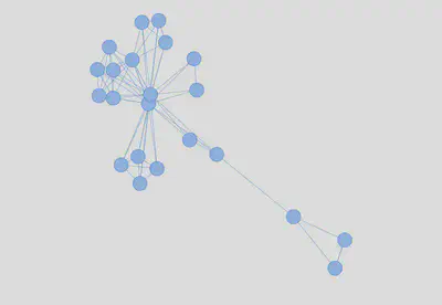
Interactive version here
This first network is not very intuitive as the nodes cannot be distinguished. Thus, I start the customization by adding some labels. These are generated with the section column followed by the first 20 characters of the title column:
nodes$label <- paste0(nodes$section, ":\n", ifelse(nchar(nodes$title) >20, paste0(substr(nodes$title,1,20), "..."), nodes$title))

visNetwork::visNetwork(nodes, edges)%>%
  visNetwork::visIgraphLayout(layout = "layout_nicely",randomSeed = 666)%>%
  visNetwork::visOptions(highlightNearest = list(hover = T))
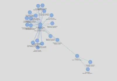
Interactive version here
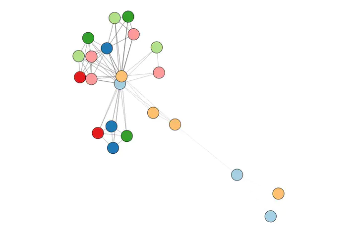
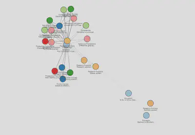
Even with labels the network is still not very intuitive. What if I add some colour? For instance, I can colour each node by the section it belongs to. For this network I selected the Paired color palette from RColorBrewer. This allows me to pair by colour similar sections (education and online education cours, proteomics and genomics publications, and so on) and better visualize the nodes:
#Node border color
nodes$color.border <- "black"

#Node background color
sections <- unique(nodes$section)

colors <- RColorBreIr::breIr.pal(n = length(sections), "Paired")
nodes$color.background <- nodes$section

for (i in 1:length(sections)) {

  nodes[nodes$section == sections[i],]$color.background <- colors[i]

}

visNetwork::visNetwork(nodes, edges)%>%
  visNetwork::visIgraphLayout(layout = "layout_nicely",randomSeed = 666)%>%
  visNetwork::visOptions(highlightNearest = list(hover = T))
Interactive version here
Now that our nodes look beautiful I can focus on the edges. I like to colour them in shades in grey, so they get darker as they get closer to the current year:
years <- sort(unique(edges$year))

colors <- RColorBreIr::breIr.pal(n = length(years), "Greys")

edges$color <- as.character(edges$year)

for (i in 1:length(years)) {

  edges[edges$year == years[i],]$color <- colors[i]

}

visNetwork::visNetwork(nodes, edges)%>%
  visNetwork::visIgraphLayout(layout = "layout_nicely",randomSeed = 666)%>%
  visNetwork::visOptions(highlightNearest = list(hover = T))
Interactive version here
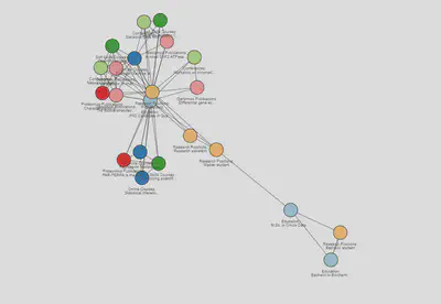
For the static version of the network that would be it. I have now an intuitive network that shows in a nice flow on my career path. Hooray!
There are a couple more twitches I like to perform for the interactive version:
- Change the colour of selected node
- Remove the labels, as you can hoover over the node to check its name
#Remove labels
nodes <- nodes %>% dplyr::select(-label)

#Highlight selected node in black
visNetwork::visNetwork(nodes, edges)%>%
  visNetwork::visIgraphLayout(layout = "layout_nicely",randomSeed = 666)%>%
  visNetwork::visNodes(color = list(highlight = "black"))%>%
  visNetwork::visOptions(highlightNearest = list(hover = T))
This gives our final interactive CV network which, again, can be explored here.
I hope you liked this plot and tutorial!